Why the same defect count can produce different yield
Die yield is the fraction of evaluated dies that meet a stated acceptance criterion. A defect counter measures a different quantity. A particle may land where it causes no electrical failure, while a small defect in a sensitive location can disable a circuit. A useful first model therefore connects defect density to critical area, the area vulnerable to the specified defect mechanism, rather than treating every detected particle as a failed die.
This article explains a random-defect model. It does not estimate a foundry's yield, prescribe a process limit, or replace electrical testing.
Process checkpoint
Understand TiN/Ti CMP in context
Distinguish conductive field residue, tungsten recess and dielectric loss in the CMP lesson; do not infer a calibrated yield from any single defect count.
Process context for “Die Yield, Defect Density and Critical Area: Read the Model”: 40nm BSI CMOS Image Sensor · CONTACT · Step 124
Read the model before using the number
For independent, randomly distributed killer defects, the elementary Poisson model is:
Y = exp(-D × A_c)
Here, D is the density of defects relevant to the modeled failure and A_c is the associated critical area. Use compatible area units. Their product is dimensionless and represents the expected number of those defects in the critical area. Y is the probability of zero such defects. The model does not imply that all failures originate from that mechanism.
The critical area need not equal the drawn die area. It depends on which defect and layout interaction is being considered. A conductive bridge between two intended separate nets and an isolated conductive speck outside sensitive geometry do not have the same consequence. The distinction is about location and failure mechanism, not whether a defect looks large in an image.
A dimensionless comparison
The following values are calculated teaching examples, not measured production data. Set λ = D × A_c so no manufacturing density or feature size is prescribed.
| Case | Expected killer defects λ | Probability of zero, exp(-λ) |
|---|---|---|
| A | 0.1 | 0.905 |
| B | 0.5 | 0.607 |
| C | 1.0 | 0.368 |
Compare A and B: the change is in the expected defect count in the sensitive area. The calculation alone cannot say whether the difference came from contamination, layout sensitivity, or both. At fixed D, doubling A_c changes Y to Y². At fixed A_c, halving D gives the square root of the original Y. These are consequences of this equation, not universal yield improvement guarantees.
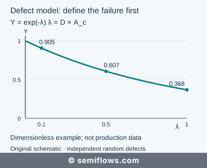
Original concept schematic; not a course cross-section or manufacturing recipe.
Where this model stops
Defects can cluster rather than occur independently. Systematic pattern failures can repeat at the same geometry. Electrical limits can fail even when no counted particle is present. These situations require different evidence and potentially different models. The textbook presents alternatives to the Poisson assumption and distinguishes module-level from total-flow defect contributions. Multiplying module yields also needs an independence assumption.
A useful counterexample is a repeated lithographic bridge at one vulnerable pattern. Calling it a uniform random-defect density hides the repeatable cause. Another is counting every surface particle and inserting that number into D without checking detection sensitivity or whether those particles can cause the modeled failure.
Work the problem
Two hypothetical layouts have the same die area. Layout A has a larger critical area for a particular bridging defect. At equal relevant defect density, which has the lower model yield? A, because its D × A_c is larger. Equal die area does not establish equal critical area.
Now suppose both layouts show the same counted surface particles, but electrical failure maps differ. Before blaming a single process, ask: are the particle measurement and electrical test from comparable stages; which counted defects can cause this failure; and is the spatial pattern random, clustered, or repeated? Record the missing evidence instead of forcing a yield estimate.
For a concrete failure-path exercise, open the field-barrier CMP step in the 40nm CIS flow. Distinguish conductive field residue, plug recess, and dielectric loss. These are different mechanisms; the step does not provide a calibrated die-yield model. Its public preview is available anonymously, with the complete lesson available after free sign-in.
The manufacturing process map places this discussion within a complete fabrication sequence. Neither a successful individual step nor a high model probability certifies final die acceptance.
Sources
Plummer, Deal and Griffin, Silicon VLSI Technology, section 4.5.1, pp. 162–164. ISBN 978-0130850379. The source supplies the model assumptions and critical-area distinction; the dimensionless examples and exercise are calculated here.
References
Silicon VLSI Technology - Full
James D. Plummer, Michael D. Deal, Peter B. Griffin
Silicon VLSI Technology · ISBN 978-0130850379